Class

A class for representing polygons composed of multiple contours, some of which may be holes.

Objects from the Class

Objects can be created by calls of the form new("gpc.poly", ...) or by reading in from a file using read.polyfile.

Slots

pts: Object of class “list”. Actually, pts is a list of lists with length equal to the number of contours in the "gpc.poly" object. Each element of pts is a list of length 3 with names x, y, and hole. x and y are vectors containing the x and y coordinates, respectively, while hole is a logical indicating whether or not the contour is a hole.

Methods

[: signature(x = "gpc.poly"): ...
append.poly: signature(x = "gpc.poly", y = "gpc.poly"): ...
area.poly: signature(object = "gpc.poly"): ...
coerce: signature(from = "matrix", to = "gpc.poly"): ...
coerce: signature(from = "data.frame", to = "gpc.poly"): ...
coerce: signature(from = "numeric", to = "gpc.poly"): ...
coerce: signature(from = "list", to = "gpc.poly"): ...
coerce: signature(from = "SpatialPolygons", to = "gpc.poly"): ...
coerce: signature(from = "gpc.poly", to = "matrix"): ...
coerce: signature(from = "gpc.poly", to = "numeric"): ...
coerce: signature(from = "gpc.poly", to = "SpatialPolygons"): ...
get.bbox: signature(x = "gpc.poly"): ...
get.pts: signature(object = "gpc.poly"): ...
intersect: signature(x = "gpc.poly", y = "gpc.poly"): ...
plot: signature(x = "gpc.poly"): The argument poly.args can be used to pass a list of additional arguments to be passed to the underlying polygon call.
scale.poly: signature(x = "gpc.poly"): ...
setdiff: signature(x = "gpc.poly", y = "gpc.poly"): ...
show: signature(object = "gpc.poly"): Scale x and y coordinates by amount xscale and yscale. By default xscale equals yscale.
symdiff: signature(x = "gpc.poly", y = "gpc.poly"): ...
union: signature(x = "gpc.poly", y = "gpc.poly"): ...
tristrip: signature(x = "gpc.poly"): ...
triangulate: signature(x = "gpc.poly"): ...

Author

Roger D. Peng

Note

The class "gpc.poly.nohole" is identical to "gpc.poly" except the hole flag for each contour of a "gpc.poly.nohole" object is always FALSE.

Examples

## Make some random polygons
set.seed(100)
a <- cbind(rnorm(100), rnorm(100))
a <- a[chull(a), ]

## Convert `a' from matrix to "gpc.poly"
a <- as(a, "gpc.poly")

b <- cbind(rnorm(100), rnorm(100))
b <- as(b[chull(b), ], "gpc.poly")

## More complex polygons with an intersection
p1 <- read.polyfile(system.file("poly-ex-gpc/ex-poly1.txt", package = "rgeos"))
p2 <- read.polyfile(system.file("poly-ex-gpc/ex-poly2.txt", package = "rgeos"))

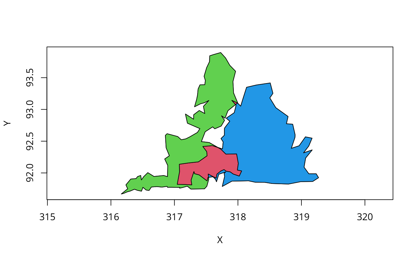
## Plot both polygons and highlight their intersection in red
plot(append.poly(p1, p2))
plot(intersect(p1, p2), poly.args = list(col = 2), add = TRUE)
#> Warning: GEOS support is provided by the sf and terra packages among others
#> Warning: implicit list embedding of S4 objects is deprecated

## Highlight the difference p1 \ p2 in green
plot(setdiff(p1, p2), poly.args = list(col = 3), add = TRUE)
#> Warning: GEOS support is provided by the sf and terra packages among others
#> Warning: implicit list embedding of S4 objects is deprecated

## Highlight the difference p2 \ p1 in blue
plot(setdiff(p2, p1), poly.args = list(col = 4), add = TRUE)
#> Warning: GEOS support is provided by the sf and terra packages among others
#> Warning: implicit list embedding of S4 objects is deprecated


## Plot the union of the two polygons
plot(union(p1, p2))
#> Warning: GEOS support is provided by the sf and terra packages among others
#> Warning: implicit list embedding of S4 objects is deprecated


## Take the non-intersect portions and create a new polygon
## combining the two contours
p.comb <- append.poly(setdiff(p1, p2), setdiff(p2, p1))
#> Warning: GEOS support is provided by the sf and terra packages among others
#> Warning: implicit list embedding of S4 objects is deprecated
#> Warning: GEOS support is provided by the sf and terra packages among others
#> Warning: implicit list embedding of S4 objects is deprecated
plot(p.comb, poly.args = list(col = 2, border = 0))


## Coerce from a matrix
x <- 
structure(c(0.0934073560027759, 0.192713393476752, 0.410062456627342, 
0.470020818875781, 0.41380985426787, 0.271408743927828, 0.100902151283831, 
0.0465648854961832, 0.63981588032221, 0.772382048331416,
0.753739930955121, 0.637744533947066, 0.455466052934407,
0.335327963176065, 0.399539700805524, 
0.600460299194476), .Dim = c(8, 2))
y <- 
structure(c(0.404441360166551, 0.338861901457321, 0.301387925052047, 
0.404441360166551, 0.531852879944483, 0.60117973629424, 0.625537820957668, 
0.179976985040276, 0.341542002301496, 0.445109321058688,
0.610817031070196, 0.596317606444189, 0.459608745684695,
0.215189873417722), .Dim = c(7, 2))

x1 <- as(x, "gpc.poly")
y1 <- as(y, "gpc.poly")

plot(append.poly(x1, y1))
plot(intersect(x1, y1), poly.args = list(col = 2), add = TRUE)
#> Warning: GEOS support is provided by the sf and terra packages among others
#> Warning: implicit list embedding of S4 objects is deprecated


## Show the triangulation
#plot(append.poly(x1, y1))
#triangles <- triangulate(append.poly(x1,y1))
#for (i in 0:(nrow(triangles)/3 - 1)) 
#    polygon(triangles[3*i + 1:3,], col="lightblue")